Educational – Page 2

High potency cannabis and the risk of psychosis

Posted on April 24, 2015April 2, 2015 by meryemgrabski

By Eleanor Kennedy @Nelllor_

This blog originally appeared on the Mental Elf site on 24th March 2015

Smoking higher-potency cannabis may be a considerable risk factor for psychosis according to research conducted in South London (Di Forti, et al., 2015).

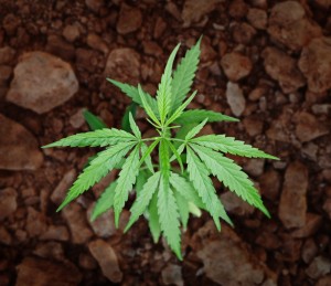
Cannabis is the most widely used illicit drug in the UK and previous research has suggested an association between use of the drug and psychosis, however the causal direction and underlying mechanism of this association are still unclear.

This recent case-control study published in Lancet Psychiatry, aimed to explore the link between higher THC (tetrahydrocannabinol) content and first episode psychosis in the community.

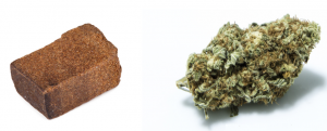
To compare the impact of THC content on first episode psychosis, participants were asked whether they mainly consumed skunk or hash. Analysis of seized cannabis suggests that skunk has THC content of between 12-16%, while hash has a much lower THC content ranging from 3-5% (Potter, Clark, & Brown, 2008; King & Hardwick, 2008).

Cannabis hash and skunk have very different quantities of the active THC component.

Methods

The researchers used a cross-sectional case-control design. Patients presenting for first-episode psychosis were recruited from a clinic in the South London and Maudsley NHS Foundation Trust; patients who had an identifiable medical reason for the psychosis diagnosis were excluded. Control participants were recruited from the local area using leaflets, internet and newspaper adverts. There were 410 case-patients and 370 controls recruited.

Researchers gathered data on participants’ cannabis use in terms of lifetime history and frequency of use as well as type of cannabis used, i.e. skunk or hash. Participants were also asked about their use of other drugs including alcohol and tobacco, as well as providing demographic information.

Results

The case-patients and control participants were different in a couple of key areas (note: psychosis is more common in men and in ethnic minorities):

	Case patients	Control participants
Male	66%	56%
Age	27.1 years	30.0 years
Caribbean or African ethnic origin	57%	30%
Completed high level of education	57%	90%
Ever been employed	88%	95%
Lifetime history of ever using cannabis	67%	63%

Participants with first episode psychosis were more likely to:

Use cannabis every day
Use high-potency cannabis
Have started using cannabis at 15 years or younger
Use skunk every day

A logistic regression adjusted for age, gender, ethnic origin, number of cigarettes smoked, alcohol units, and lifetime use of illicit drugs, education and employment history showed thatcompared to participants who had never used cannabis:

Participants who had ever used cannabis were not at increased risk of psychosis
Participants who had used cannabis at age 15 were at moderately increased risk of psychotic disorder
People who used cannabis or skunk everyday were roughly 3 times more likely to have diagnosis of psychotic disorder

A second logistic regression was carried out to explore the effects of a composite measure of cannabis exposure which combined data on the frequency of use and the type of cannabis used.Compared with participants who had never used cannabis:

Individuals who mostly used hash (occasionally, weekends or daily) did not have any increased risk of psychosis
Individuals who smoked skunk less than once a week were nearly twice as likely to be diagnosed with psychosis
Individuals who smoked skunk at weekends were nearly three times as likely to be diagnosed with psychosis
Individuals who smoked skunk daily were more than five times as likely to be diagnosed with psychosis

The population attributable factor (PAF) was calculated to estimate the proportion of disorder that would be prevented if the exposure were removed:

19.3% of psychotic disorders attributable to daily cannabis use
24.0% of psychotic disorders attributable to high potency cannabis use
16.0% of psychotic disorders attributable to skunk use every day

These findings raising awareness among young people of the risks associated with the use of high-potency cannabis

Conclusions

The results of this study support the theory that higher THC content is linked with a greater risk of psychosis, with daily use of skunk conferring the highest risk. Recruiting control participants from the same area as the case participants meant that the two groups were more likely to be matched on not only demographic factors but also in terms of the actual cannabis that both groups were consuming.

The study has some limits, such as the cross-sectional design which cannot be used to establish causality. Also the authors have not included any comparison between those who smoke hash and those who consume skunk so no conclusions can be drawn about the relative harm of hash.

Media reports about the study have mainly focussed on the finding that ‘24% of psychotic disorders are attributable to high potency cannabis use’. This figure was derived from a PAF calculation which assumes causality and does not allow for the inclusion of multiple, potentially interacting, risk factors. Crucially the PAF depends on both the prevalence of the risk factor and the odds ratio for the exposure; the PAF can be incredibly high if the risk factor is common in a given population.

In this case, the prevalence rate of lifetime cannabis use was over 60% in both participant groups. According to EMCDDA, the lifetime prevalence of cannabis use in the UK is 30% among adults aged 15-64, so it is arguable that this study sample is not representative of the rest of the UK. The authors themselves note that “the ready availability of high potency cannabis in south London might have resulted in a greater proportion of first onset psychosis cases being attributed to cannabis use than in previous studies”, which is a more accurate interpretation than media reports claiming that “1 in 4 of all new serious mental disorders” is attributable to skunk use.

Future studies looking at the relationship between cannabis and psychosis should also aim to differentiate high and low potency cannabis. Longitudinal cohort studies are particularly useful as they have the same advantages as a case-control design but data about substance use could be more reliable as ‘lifetime use’ can be gathered from multiple measurements collected at a number of time points across the lifetime.

This innovative study is the first to distinguish between different strengths of cannabis in this way.

Links

Primary study

Di Forti M. et al (2015). Proportion of patients in south London with first-episode psychosis attributable to use of high potency cannabis: a case-control study (PDF). The Lancet Psychiatry, 2(3), 233-238.

Other references

King L, & Hardwick S. (2008). Home Office Cannabis Potency Study (PDF). Home Office Scientific Development Branch.

Potter DJ, Clark P, & Brown MB. (2008). Potency of Delta(9)-THC and other cannabinoids in cannabis in England in 2005: Implications for psychoactivity and pharmacology (PDF). Journal of Forensic Sciences, 53(1), 90-94.

Screening of A Royal Hangover: TARG goes to the movies

Posted on April 15, 2015April 15, 2015 by meryemgrabski

By David Troy @DavidTroy79

I recently hosted a documentary screening of ‘A Royal Hangover’ on behalf of the Tobacco and Alcohol Research Group at the University of Bristol. The film documents anecdotes from all facets of the drinking culture in the UK, from politicians to police, medical specialists to charities, the church and scientists, and addicts and celebrities, with high profile personalities such as Russell Brand and controversial figures such as sacked Government Drugs Advisor Professor David Nutt. The director Arthur Cauty kindly agreed to take part in a question and answer session after the film to discuss his experience making the film and debate the issues raised in the film.

The film begins with Arthur talking about his own relationship with alcohol (or his lack of one). He preferred to shoot silly films, play music or wrestle than go out drinking with his friends. The film deals with the history of alcohol starting off in the 16^th and 17^th century when it was safer to drink beer than water. Even babies were given what was called “small beer for small people”. In the early 18^th century, gin became the drink of choice and reached epidemic levels, famously depicted in William Hogarth’s ‘Gin Lane’. Gin was unregulated and sold not just in public houses but in general stores and on the street. Moving on to the 20^th century, Lloyd George recognised the danger of alcohol to the war effort in World War 1, and was quoted as saying that “we are fighting Germany, Austria and drink; and as far as I can see, the greatest of these deadly foes is drink”. Around this time, restrictions on the sale of alcohol were introduced by government. During World War 2, beer was seen as important to morale and a steady supply of it was seen as important to the war effort. Since then, we have seen a steady increase in consumption levels through the ‘hooligan/lager lout’ phenomenon of the 1980’s and the binge drinking of the 1990’s and the early 2000’s. Consumption levels have been falling slightly since the mid 2000’s but there are still 10 million people drinking above the government’s recommended level.

During the film, Arthur investigates how different societies treat alcohol. French and American drinkers describe a more reserved and responsible attitude to alcohol. This is somewhat contradicted by 2010 data in a recent report by the World Health Organisation which reports that French people over the age of 15 on average consume 12.2 litres of pure alcohol a year compared to Britons at 11.6 and Americans at 9.2 litres respectively. The drinking culture of France and the United States is certainly different to that of the UK. The French consume more wine, less beer, and tend to drink alcohol whilst eating food. The US (outside of ‘Spring Break’ culture) is more disapproving of public intoxication. However, neither society should be held up as a gold standard when it comes to alcohol use.

The film talks about the enormous cost of alcohol to England; approximately £21 billion annually in healthcare (£3.5 billion), crime (£11 billion) and lost productivity (£7.3 billion) costs. These are the best data available, but costs of this nature are difficult to calculate. Arthur talked to professionals on the front line – he interviewed a GP who said that a huge proportion of her time is devoted to patients with alcohol problems and their families. She has to treat the “social and psychological wreck” that comes when one family member has an alcohol addiction. A crime commissioner from Devon and Cornwall police states that 50% of violence is alcohol-related in his area.

The film attempts to understand the reasons why alcohol use is at current levels, and offers some possible solutions. Alcohol is twice as affordable now as in the 1980’s and is more freely available than ever. This needs to be curtailed. Evidence suggests that alcoholic beverages were 61% more affordable per person in 2012 than in 1980, and the current number of licensed premises in England and Wales is at the highest level recorded in over 100 years. Licensed premises with off sales only alcohol licences have also reached a record high, more than doubling in number compared with 50 years ago. The evidence shows that price increases and restrictions on availability are successful in reducing alcohol consumption. More alcohol education in schools was highlighted as being necessary. The evidence suggests that alcohol education in schools can have some positive impact on knowledge and attitudes. Overall, though, school-based interventions have been found to have small or no effects on risky alcohol behaviours in the short-term, and there is no consistent evidence of longer-term impact. Alcohol education in schools should be part of the picture but other areas may prove more fruitful. The film suggests that parental and peer attitudes towards alcohol affect drinking norms, and these attitudes need to change. In multiple surveys, it has been found that the behaviour of friends and family is the most common influential factor in determining how likely and how often a young person will drink alcohol. Alcohol marketing was cited as a problem and it needs to regulated more stringently. Alcohol marketing increases the likelihood that adolescents will start to use alcohol and increases the amount used by established drinkers, according to a report commissioned by the EU. The exposure of children to alcohol marketing is of current concern. A recent survey showed that primary school aged children as young as 10 years old are more familiar with beer brands, than leading brands of biscuits, crisps and ice-cream.

David Nutt discussed research he conducted with colleagues, which assessed the relative harms of 20 drugs, including both harms to the individual and to others. They found that alcohol was the most harmful drug overall. Professor Nutt also covered the circumstances surrounding his sacking as government’s chief drug advisor; he claimed that ecstasy and LSD were less dangerous than alcohol, which led to his dismissal. This highlights the inherent tension between politics and science. Evidence can diverge from government policy and popular opinion, and scientists can lose their positions when reporting evidence that is politically unpopular. In my view, the reluctance of governments to implement evidence-based alcohol policies is frustrating; minimum unit pricing (MUP) being the latest example. Despite good evidence supporting how MUP can reduce alcohol-related harms, lobbying by the alcohol industry has halted its progress.

The film deals with the human cost of alcohol misuse, with personal stories of addiction permeating the film. Carrie Armstrong (who writes a blog discussing her battle with alcohol addiction), as well as Persia Lawson and Joey Rayner (who write a lifestyle blog ‘Addictive Daughter’), discussed the havoc alcohol caused in their lives, and explained how young men and women come to them for help with their own alcohol dependencies. Russell Brand talked about his own alcohol addiction during the film. He contends that his drug and alcohol use was medicinal and thinks that alcohol and drug addicts “have a spiritual craving, a yearning and we don’t the language, we don’t have the code to express that in our society”. Arthur interviewed Chip Somers of Focus 12, who talked about the low levels of funding to treat alcohol addiction. Only a small minority (approximately seven per cent) of the 1.6 million alcohol dependants in the UK can get access to treatment compared to two-thirds of addicts of other drugs.

Arthur recorded over 100 hours of footage of drinkers on nights out during the course of filming. He described it as follows: “As the sun goes down, society fades away and what emerges from the shadows is a monster of low inhibition, aggression and casual chaos”. He sums it up as us “going to war on ourselves. On one side is the police, the emergency services, the council and various groups of volunteers and on the other side you’ve got everybody else”. He was assaulted three times and witnessed multiple scenes of violence close up. His bravery is admirable – there were many scenes I found difficult to watch. The scenes of senseless violence were horrible to look at, as were the images of individuals who were so intoxicated as to be helpless and in need of medical attention.

The Q&A after the screening was quite illuminating. Arthur spoke about the reception the film has been receiving at home and abroad. The reception has been great in the United States, where the film has had successful showings at film festivals. The interest in the UK has been a little disappointing, however, which Arthur puts down to the reluctance of society at large to acknowledge our dysfunctional relationship with alcohol. Nevertheless, there has been positive feedback from viewers of the film. Many people have contacted Arthur to tell him how the film has opened their eyes to their own relationship with alcohol and prompted them to make a change. The audience was keen to engage in the conversation. One person, who has a family member with an alcohol addiction, said how important it is to raise awareness of these issues. Another person called for policy measures to be implemented such as MUP to curb use across the population.

Arthur came across as someone who is acutely aware of the damage alcohol is causing in the UK, and is doing what he can to raise the public’s consciousness about it. He has presented a unique look at booze Britain, in equal parts shocking, hilarious, sympathetic and thought provoking – a film we can all relate to. It was a very enjoyable and informative evening and I hope the audience took something away from it. I believe the arts and sciences need to work together to improve how knowledge is communicated. It was my hope that by showing this documentary, information on alcohol harms in society would be more accessible to a general audience. Change begins with the acknowledgement of new information that alters the view of ourselves and our behavior. It has been estimated that over 7 million people in the UK are unaware of the damage their personal alcohol use is doing. I believe the blame lies on both sides. Alcohol researchers need to communicate the harms of alcohol in more engaging and accessible ways and members of the general public need to seek out such information. All too often scientists get the reputation as being cold, boring, and amoral. Collaborating with filmmakers and other proponents of the arts on events such as the one I hosted can assist in changing that stereotype.

Is moderate alcohol consumption good for you?

Posted on April 13, 2015April 2, 2015 by meryemgrabski

By Marcus Munafo @MarcusMunafo

This blog originally appeared on the Mental Elf site on 13th March 2015

This is something many of us would like to be true – the idea that the occasional glass of wine has health benefits is compelling in a society like the UK where alcohol consumption is widespread.

Certainly the observational data indicate a J-shaped associationbetween alcohol consumption and mortality (O’Keefe et al, 2007), with the lowest mortality observed at low to moderate levels of alcohol consumption (equivalent to perhaps a pint of beer a day for men, and about half that for women).

However, observational studies like this are fraught with difficulties.

First, people may not report their alcohol consumption reliably.
Second, and more importantly, alcohol consumption is associated with a range of other lifestyle behaviours, such as diet and smoking, which will themselves influence mortality, so that isolating any specific association of alcohol is extremely difficult.
Third, how non-drinkers are defined may be important – lifetime abstainers may be different from former drinkers (who could have stopped drinking because of health problems).

The last point illustrates the problem of reverse causality; alcohol consumption may be causally associated with a range of health outcomes, but some of those health outcomes may also be causally associated with alcohol consumption.

In a recent study in the BMJ, the authors argue that the problems associated with the choice of an appropriate referent group of non-drinkers are often overlooked in research into alcohol-related mortality.

They also argue that age is not adequately considered, which may be relevant because of physiological changes to the ageing body that influence elimination of blood alcohol. Knott and colleagues explored the association between alcohol consumption and all cause mortality for people aged less than 65 years and aged 65 or more, and separated never and former drinkers.

Methods

The authors used data from the Health Survey for England, an annual, nationally-representative cross sectional survey of the general population, linked to national mortality registration data.

The analysis focused on adults aged 50 years or older, and investigated two measures of alcohol consumption: self-reported average weekly consumption over the past year, and self-reported consumption on the heaviest day in the past week. The outcome was all cause mortality (i.e., any death recorded during the period of data collection).

The primary statistical analyses were proportional hazards analyses for each of the two age groups of interest (less than 65 years and 65 years or more). They tested for whether any associations observed differed between males and females and, given strong evidence of a sex-dose interaction, reported sex-specific models for each age group of interest.

Statistical adjustment was made for a comprehensive list of potential confounders, such as geographical location, ethnicity, cigarette smoking, obesity and a range of socio-demographic variables.

Results

Protective associations were only observed with statistical significance (a point I’ll return to below) among younger men (aged 50 to 64 years) and older women (65 years or older), using a never drinker referent category after full adjustment.

Among younger men a protective relationship between alcohol consumption and all cause mortality was observed among those who reported consuming 15.1 to 20 units per week (hazard ratio 0.49, 95% confidence interval 0.26 to 0.91).

Among older women, the range of protective use was broader but lower, with reductions in hazards of all cause mortality observed at all consumption levels up to 10 units per week of less.

The study supports a moderate protective effect of alcohol.

Conclusions

The authors conclude that observed associations between low levels of alcohol consumption and reduced all cause mortality may in part be due to inappropriate selection of a referent group (all non-drinkers, rather than never drinkers) and inadequate statistical adjustment for potential confounders.

They also conclude that beneficial dose response relationships between alcohol consumption and all cause mortality may be specific to women aged 65 years or older.

There is a relative lack of data on older populations in relation to the association between alcohol consumption and all cause mortality, which this study addresses. The consideration of different definitions of the referent category is also valuable – the authors are correct that conventional definitions of “non-drinker” may be problematic.

However, to what extent should we believe the conclusion that beneficial dose response relationships may be age- and sex-specific?

As David Spiegelhalter has pointed out, the authors base their conclusion on which associations achieved statistical significance and which did not. However, the hazard ratios for all cause mortality are consistently lower for alcohol consumers than non-consumers in this study. Although the confidence intervals are wider for some consumption levels and in some sub-groups (males vs females, or younger vs older), the individual hazard ratios are all consistent with each other.

The wide confidence intervals reflect a lack of statistical power, principally due to the small number of never drinkers, and the small number of deaths. Although the data set is relatively large, by carving it up into a number of sub-groups, the statistical power for the individual comparisons is reduced. Spiegelhalter points out that the entire comparison for participants in the younger age group is based on 17 deaths in the male baseline group and 19 deaths in the female group.

As Andrew Gelman and Hal Stern have said, the difference between “significant” and “non-significant” is not (necessarily) itself significant. Indeed, focusing on statistical significance (rather than effect size and precision) can lead to exactly the problems encountered here. Low statistical power is also a problem, reducing the likelihood that a statistically significant finding is true, and (perhaps more importantly) dramatically reducing the precision of our effect size estimates.

Strengths and limitations

There are some strengths to this study, notably the use of a more considered referent category of never drinkers, and the statistical adjustment for a broad range of potential confounders.

However, the primary conclusion of the authors does not seem to be borne out by their own data – hazard ratios for all cause mortality are lower for alcohol consumers than non-consumers at all levels of consumption, for both men and women, and for both the younger and older age groups.

Is moderate alcohol consumption good for us then? The observational data, including that from this study, continues to suggest so.

However we should also remain wary of evidence from observational studies, which can be notoriously unreliable, and cannot confirm that an association is causal. Ultimately, we may need to use novel methods to answer this question, such as Mendelian randomization which utilized the properties of genetic variants to enable stronger causal inference.

We should be wary of evidence from observational studies, which can be notoriously unreliable, especially in underpowered studies like this one.

Link

Knott CS, Coombs N, Stamatakis E, Biddulph JP. (2015) All cause mortality and the case for age specific alcohol consumption guidelines: pooled analyses of up to 10 population based cohorts (PDF). British Medical Journal, 350, h384. doi: 10.1136/bmj.h384

O’Keefe HF, Bybee KA, Lavie CJ. (2007) Alcohol and cardiovascular health: the razor-sharp double-edged sword. J Am Coll Cardiol. 2007;50(11)

Spiegelhalter D. (2015) Misleading conclusions from alcohol protection study. Understanding Uncertainty website, last accessed 11 Mar 2015.

Research Responsibly: Things to Consider when Science and Politics Meet

Posted on January 13, 2015 by meryemgrabski

By Meryem Grabski

It might not come as a surprise that doing a PhD is not always fun. One thing that gets me through those difficult, yet inevitable, times is the idea that the research I am doing could potentially make a difference for the better. I am sure this is true for many people involved in research fields that touch upon big societal questions such as health, climate change, economics, or education.

Surprisingly though, I realized a little while ago that I have given little thought to how relevant findings make their way to those who implement societal changes, such as policy makers. Usually scientists are trained to communicate their findings to other scientists, not politicians (or the general public, the people that empower the policy makers in the first place, but I will leave this important issue to one side for now). So what should scientific advice to policy makers look like? Is a brief summary of the research outcomes adequate or should a preference for the implementation of the findings be stated?

I started thinking about this after a discussion in our weekly lab meeting about an article published by Tamsin Edwards, a climate scientist. She describes how her refusal to give specific recommendations for political courses of action has sometimes been met with criticism – from environmentalists and members of the public, as well as fellow climate scientists. She gets accused of having a hidden political agenda, not fulfilling her role as an expert sufficiently, and failing to act and therefore delaying important and pending decisions. Even if some of these points are valid, a counter-argument could equally be made that openly stating political preferences could impact scientific impartiality and lead to the abuse of science to serve political agendas.

This complex issue is described in a model by Pielke, which characterizes four ways in which scientists can position themselves towards policy making. These roles, described in more details in Pilke’s book The Honest Broker: Making Sense of Politics and Policy are briefly summarized below, as well as their potential benefits and pitfalls.

The “pure scientists” do research for the sake of research only and have no further interest in the application of the findings. In reality, this type of “ivory tower” scientist is very rare today, especially in fields where findings might have a potential impact on society.

Pros: Maximal impartiality; because pure scientists are not interested in engaging in political decision-making, they are least likely to be biased towards one specific outcome.

Cons: Since pure scientists are not motivated to make scientific findings accessible, they are not facilitating the implementation of their findings, therefore making them useless for society. Even the publication of findings in scientific journals is often trapped behind expensive paywalls and therefore not accessible by interested members of the public.

The “issue advocates” can be placed on the other end of the continuum of involvement with politics. They believe that participating in the political decision making process is an important part of their role as a scientist. The issue advocate is dedicated to a specific political agenda or outcome, and therefore more likely to narrow the view of the advice seeker to one specific course of action, in line with their own views.

Pros: As the political opinion of the issue advocates is laid out openly, they might be less suspected of having a “hidden political agenda” (even though, in the case of “stealth advocacy”, the opposite could be the case as explained below). Acting as an expert with a specific goal in mind, an issue advocate might be more efficient in aiding policy makers with the fast implementation of findings.

Cons: Issue advocates might be more likely to be biased towards specific research outcomes (as they strongly favour one political outcome they are likely to be in a dilemma when their research findings do not support this outcome). Pielke describes the danger of “stealth issue advocacy”, which refers to a scientist hiding a political agenda while claiming to focus on the science. This usually results in scientific “facts” being manipulated for political debate. This behaviour can harm the credibility of scientific claims in general.

The “science arbiters” believe that science should not be directly involved in political decision making, but are willing to act as experts to inform policy making. Science arbiters focus on narrow, scientifically testable questions in order to stay removed from political debate.

Pros: More useful to society than “pure scientists”, as they are willing to act as scientific experts if specific questions are asked.

Cons: Science arbiters could be accused of being too passive, as they are only reacting to requests, but not actively engaging in sharing their knowledge.

The “honest broker of policy alternatives” is, as compared to the science arbiter, actively seeking to integrate scientific findings in policy decision making by providing policy makers with clarification on specific questions and presenting several alternatives of political action. The honest broker is, in contrast to the issue advocate, not interested in a specific political outcome but in simply engaging with policy decision makers in order to integrate scientific knowledge into the decision making process. Tamsin Edward’s stance towards policy making could be described as “honest brokering”.

Pros: The honest broker is a great facilitator of scientific expertise to society.

Cons: The role of the honest broker seems difficult to maintain for one person alone as they are very actively engaged in politics but at the same time have to remain completely impartial to one specific political outcome and furthermore should examine the issue from several aspects. Pielke suggests that committees and bodies of several experts could act as an honest broker together.

Pielke further elaborates on which role might be most suitable, taking into account the degree of consensus on political values and the degree of uncertainty in scientific knowledge. Admittedly the different roles described are idealized and in reality might not quite fit into this abstract framework.

I personally found two important points to take away from this discussion: Firstly, it is crucial to understand that there are different options regarding how to discuss scientific findings with policy makers. Secondly, there is no perfect one-size-fits-all approach concerning which option to choose, as each option has advantages and disadvantages. I believe that reflecting on the issue and discussing it, privately, like we did in our lab group or, like Edwards, in an open debate, are a good start to finding a personal stance towards policy making. This might seem laborious and time consuming but, in my opinion, should be integral to all scientists, who pride themselves with doing science that matters.

The missing heritability problem

Posted on November 18, 2014October 20, 2014 by Marcus Munafo

By Marcus Munafo

Missing heritability has been described as genetic “dark matter”In my last post I described the transition from candidate gene studies to genome-wide association studies, and argued that the corresponding change in the methods used, focusing on the whole genome rather than on a handful of genes of presumed biological relevance, has transformed our understanding of the genetic basis of complex traits. In this post I discuss the reasons why, despite this success, we still have not accounted for all the genetic influences we expect to find.

As I discussed previously, genome-wide association studies (GWAS) have been extremely successful in identifying genetic variants associated with a range of disease outcomes – countless replicable associations have emerged over the last few years. Nevertheless, despite this success, the proportion of variability in specific traits accounted for so far is much less than what twin, family and adoption studies would lead us to expect. The individual variants identified are associated with a very small proportion of variance in the trait of interest (typically 0.1% of less), so that together they still only account for a modest proportion. Twin, family and adoption studies would lead us to expect that 50% or more of the variance in many complex traits is attributable to genetic influences, but so far we have found only a small fraction of that total. This has become known as the “missing heritability” problem. Where are the other genes? Should we be seeking common genetic variants of smaller and smaller effect, in larger and larger studies? Or is there a role for rare variants (i.e., those which occur with a low frequency in a particular population, typically a minor allele frequency less than 5%), which may have a larger effect?

It is clear that some missing heritability will be accounted for by variants that have not yet been identified via GWAS. Most GWAS genotyping chips don’t capture rare variants very well, but evolutionary theory predicts that those mutations that strongly influence complex phenotypes will tend to occur at low frequencies. Under the evolutionary neutral model, variants with these large effects are predicted to be rare. However, under the same model, while rare variants of large effect constitute the majority of causal variants, they still only contribute a small proportion of phenotypicvariance in a population, because they are rare. On the other hand, common variants of small effect contribute a greater overall proportion of variance. There are new methods which use a less stringent threshold for including variants identified via GWAS – instead of only including those that reach “genomewide significance” (i.e., a P-value < 10^-8 – see my earlier post), those which reach a much more modest level of statistical evidence (e.g., P < 0.5) are included. This much more inclusive approach has shown that when considered together, common genetic variants do in fact seem to account for a substantial proportion of expected heritability.

In other words, complex traits, such as most disease outcomes but also those behavioural traits of interest to psychologists, are highly polygenic – that is, they are influenced by a very large number of common genetic variants of very small effect. This, in turn, explains why we have yet to reliably identify specific genetic variants associated with many psychological and behavioural traits – while the latest GWAS of traits such as height and weight (the GIANT Consortium) includes data on over 250,000 individuals, there exists no such collection of data on most psychological and behavioural traits. This situation is changing though – a recent GWAS of educational attainment combined data on over 125,000 individuals, and three genetic loci were identified with genomewide significance, although these were associated with very small effects (as we would expect). Excitingly, these findings have recently been replicated. Another large GWAS, this time of schizophrenia, identified 108 loci associated with the disease, putting this psychiatric condition on a par with traits such as height and weight in terms of our understanding of the underlying genetics.

The success of the GWAS method is remarkable – the recent schizophrenia GWAS, for example, has provided a number of intriguing new biological targets for further study. It should only be a matter of time (and sample size) before we begin to identify variants associated with personality, cognitive ability and so on. Once we do, we will understand more about the biological basis for these traits, and finally begin to account for the missing heritability.

References:

Munafò, M.R., & Flint J. (2014). Schizophrenia: genesis of a complex disease. Nature, 511, 412-3.

Rietveld, C.A., et al. (2013). GWAS of 126,559 individuals identifies genetic variants associated with educational attainment. Science, 340, 1467-71.

@MarcusMunafo

@BristolTARG

This blog first appeared on The Inquisitive Mind site on 18th October 2014.

Having confidence…

Posted on June 10, 2013 by Marcus Munafo

I’ve written previously about the problems associated with an unhealthy fixation on P-values in psychology. Although null hypothesis significance testing (NHST) remains the dominant approach, there are a number of important problems with it. Tressoldi and colleagues summarise some of these in a recent article.

First, NHST focuses on rejection of the null hypothesis at a pre-specified level of probability (typically 5%, or 0.05). The implicit assumption, therefore, is that we are only interested answering “Yes!” to questions of the form “Is there a difference from zero?”. What if we are interested in cases where the answer is “No!”? Since the null hypothesis is hypothetical and unobserved, NHST doesn’t allow us to conclude that the null hypothesis is true.

Second, P-values can vary widely when the same experiment is repeated (for example, because the participants you sample will be different each time) – in other words, it gives very unreliable information about whether a finding is likely to be reproducible. This is important in the context of recent concerns about the poor reproducibility of many scientific findings.

Third, with a large enough sample size we will always be able to reject the null hypothesis. No observed distribution is ever exactly consistent with the null hypothesis, and as sample size increases the likelihood of being able to reject the null increases. This means that trivial differences (for example, a difference in age of a few days) can lead to a P-value less than 0.05 in a large enough sample, despite the difference having no theoretical or practical importance.

The last point is particularly important, and relates to two other limitations. Namely, the P-value doesn’t tell us anything about how large an effect is (i.e., the effect size), or about how precise our estimate of the effect size is. Any measurement will include a degree of error, and it’s important to know how large this is likely to be.

There are a number of things that can be done to address these limitations. One is the routine reporting of effect size and confidence intervals. The confidence interval is essentially a measure of the reliability of our estimate of the effect size, and can be calculated for different ranges. A 95% confidence interval, for example, represents the range of values that we can be 95% confident that the true effect size in the underlying population lies within. Reporting the effect size and associated confidence interval therefore tells us both the likely magnitude of the observed effect, and the degree of precision associated with that estimate. The reporting of effect sizes and confidence intervals is recommended by a number of scientific organisations, including the American Psychological Association, and the International Committee of Medical Journal Editors.

How often does this happen in the best journals? Tressoldi and colleagues go on to assess the frequency with which effect sizes and confidence intervals are reported in some of the most prestigious journals, including Science, Nature, Lancet and New England Journal of Medicine. The results showed a clear split. Prestigious medical journals did reasonably well, with most selected articles reporting prospective power (Lancet 66%, New England Journal of Medicine 61%) and an effect size and associated confidence interval (Lancet 86%, New England Journal of Medicine 83%). However, non-medical journals did very poorly, with hardly any selected articles reporting prospective power (Science 0%, Nature 3%) or an effect size and associated confidence interval (Science 0%, Nature 3%). Conversely, these journals frequently (Science 42%, Nature 89%) reported P-values in the absence of any other information (such as prospective power, effect size or confidence intervals).

There are a number of reasons why we should be cautious when ranking journals according to metrics intended to reflect quality and convey a sense of prestige. One of these appears to be that many of the articles in the “best” journals neglect some simple reporting procedures for statistics. This may be for a number of reasons – editorial policy, common practices within a particular field, or article formats which encourage extreme brevity. Fortunately the situation appears to be improving – Nature recently introduced a methods reporting checklist for new submissions, which includes statistical power and sample size calculation. It’s not perfect (there’s no mention of effect size or confidence intervals, for example), but it’s a start…

Reference:

Tressoldi, P.E., Giofré, D., Sella, F. & Cumming, G. (2013). High impact = high statistical standards? Not necessarily so. PLoS One, e56180.

Posted by Marcus Munafo

Shifting the Evidence

Posted on May 28, 2013 by oliviamaynard

An excellent paper published a few years ago, Sifting the Evidence, highlighted many of the problems inherent in significance testing, and the use of P-values. One particular problem highlighted was the use of arbitrary thresholds (typically P < 0.05) to divide results into “significant” and “non-significant”. More recently, there has been a lot of coverage of the problems of reproducibility in science, and in particular distinguishing true effects from false positives. Confusion about what P-values actually tell us may contribute to this.

It is often not made clear whether research is exploratory or confirmatory. This distinction is now commonly made in genetic epidemiology, where individual studies routinely report “discovery” and “replication” samples. That in itself is helpful – it’s all too common for post-hoc analyses (e.g., of sub-groups within a sample) to be described as having been based on a priori hypotheses. This is sometimes called HARKing (Hypothesising After the Results are Known), which can make it seem like results were expected (and therefore more likely to be true), when in fact they were unexpected (and therefore less likely to be true). In other words, a P-value alone is often not very informative in telling us whether an observed effect is likely to be true – we also need to take into account whether it conforms with our prior expectations.

One way we can do this is by taking into account the pre-study probability that the effect or association being investigated is real. This is difficult of course, because we can’t know this with certainty. However, what we perhaps can estimate is the extent to which a study is exploratory (the first to address a particular question, or use a newly-developed methodology) or confirmatory (the latest in a long series of studies addressing the same basic question). Broer et al (2013) describe a simple way to take this into account and increase the likelihood that a reported finding is actually true. Their basic point is that the likelihood that a claimed finding is actually true (which they call the positive predictive value, or PPV) is related to three things: the prior probability (i.e., whether the study is exploratory or confirmatory), the statistical power (i.e., the probability of finding an effect if it really exists), and the Type I error rate (i.e., the P-value or significance threshold used). We have recently described the problems associated with low statistical power in neuroscience (Button et al., 2013).

What Broer and colleagues show is that if we adjust the P-value threshold we use, depending on whether a study is exploratory or confirmatory, we can dramatically increase the likelihood that a claimed finding is true. For highly exploratory research, with a very low prior probability, they suggest a P-value of 1 × 10^-7. Where the prior probability is uncertain or difficult to estimate, they suggest a value of 1 × 10^-5. Only for highly confirmatory research, where the prior probability is high, do they suggest that a “conventional” value of 0.05 is appropriate.

Psychologists are notorious for having an unhealthy fixation on P-values, and particularly the 0.05 threshold. This is unhelpful for lots of reasons, and many journals now discourage or even ban the use of the word “significant”. The genetics literature that Broer and colleagues draw on has learned these lessons from bitter experience. However, if we are going to use thresholds, it makes sense that these reflect the exploratory or confirmatory nature of our research question. Fewer findings might pass these new thresholds, but those that do will be much more likely to be true.

References:

Broer L, Lill CM, Schuur M, Amin N, Roehr JT, Bertram L, Ioannidis JP, van Duijn CM. (2013). Distinguishing true from false positives in genomic studies: p values. Eur J Epidemiol; 28(2): 131-8.

Button KS, Ioannidis JP, Mokrysz C, Nosek BA, Flint J, Robinson ES, Munafò MR. (2013). Power failure: why small sample size undermines the reliability of neuroscience. Nat Rev Neurosci; 14(5): 365-76.

Posted by Marcus Munafo and thanks to Mark Stokes at Oxford University for the ‘Statistical power is truth power’ image.